Cooling Efficiency Algorithms: Air-Side Economizers and Temperature Differentials25 min read

I prefer the term “economizer” to “free cooling” for obvious enough reasons: It’s not free. Even air-side economization does not merely require opening the windows. Beyond fans to evacuate hot air and capture and distribute cooling air, we have humidity management and contamination management, both of which require monitoring as well as control. I started this series on cooling efficiency algorithms last September to provide a roadmap for removing some of the guesswork in both design decisions and management practices in the data center. By dribbling these out in discrete blog-bites, I hope to have kept the subject alive for readers who might otherwise not feel inclined to self-indulgently tackle a long white paper or text book. In a subset of these algorithms I have addressed series water-side economization1 and parallel water-side economization.2 In today’s piece, I will present algorithms for assessing the relative merits of air-side economization in terms compatible with the previous discussions. Upon completion of this series, we will apply these algorithms to a couple different scenarios to explore the variables which might make one model more attractive than another.
For any readers who missed the previous pieces in this series, I am presenting every economization option in terms of a common baseline which will then allow us to make some apples-to-apples comparisons when we finally wrap this up. Therefore, I am assuming a data center with excellent airflow management practices in place that allow us to have a 76˚F supply air temperature capable of providing server inlet temperatures in a 76-78˚F range. With that 76˚F supply temperature, we can see in the sample cities in Figure 1 that different types of economization will give us access to different proportions of economization in different climate zones. Nevertheless, access to hours does not necessarily directly correlate to energy use, hence the algorithm tools I have developed and am sharing.
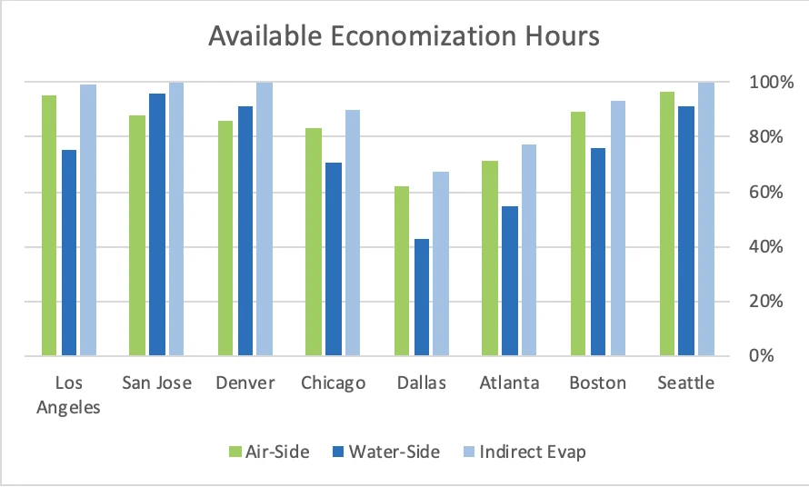
Figure 1: Access to Economization for Sample Cities, at 76˚F Supply Temperature
While my assumption about airflow management best practices and the resultant set point management flexibility may not change the relative merits of different variations of economization, it definitely moves the needle on whether or not economization should even be considered. Figure 2 illustrates access to economization hours at different levels of airflow management. Remember, before airflow management was everybody’s favorite topic at poker parties, BBQs, and happy hours, we saw return air set points around 68-70˚F, resulting in supply air temperatures in the 50-55˚F range. Therefore, the worst case number in Figure 2 (58˚F) still represents racks arranged in hot aisle – cold aisle and maybe some floor grommets and blanking panels deployed with random inconsistency, thereby allowing a 75˚F set-point resulting in 58˚F supply. Regardless, the economization hours data suggests pretty strongly that with less than optimum airflow management, an investment in economization is going to be difficult to justify. With good airflow management, such investments are clearly in the no-brainer category.
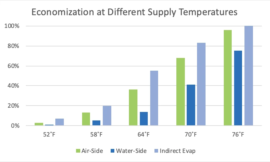
Figure 2: Economization at Different Supply Air Temperatures, Los Angeles Example
As with previous discussions, building an operating budget for air-side economization requires reliable data for making meaningful comparisons between different economization alternatives and forecasting return on investment for those alternatives. Most of the data requirements are going to be the same, though air-side will work with dry bulb temperatures and we will also want to work with dew point data. Specifically, the air-side algorithms will require:
Supply air temperature
Ambient temperature – dry bulb (DB)
Ambient humidity (dew point)
Economizer fan energy
Humidification energy
De-humidification energy
Mechanical plant energy when not in economizer mode
Hourly climate history data is available from various sources in various forms. Personally, I have organized data for several hundred NOAA stations in look-up tables that look like Table 1 below. Each cell in the Hours WB< and Hours DB< columns looks something like this: =IF(F724<$Q$9,1,0), so I can just reference the column header cells into any equation and it will calculate hours for any value I apply. There will be 8760 lines in each look up table. Be sure to closely scrutinize all the data you purchase. Not all weather stations are absolutely diligent in maintaining complete records. I guarantee you will find lines with no data recorded. My suggestion for when you encounter these omissions is to enter values that fall halfway between the preceding data point and subsequent data point. While these estimates may cause you to miss some outliers, such as 1:53 am and 4:53 am in Table 1, the resultant exponential smoothing will still be more accurate than calculating all zeros for missing data points. Such tables were integral to the algorithms I developed for series water-side economization and parallel water-side economization. Making dew point data useful gets a little more interesting. One approach could be to add a whole row of additional columns to Table 1 to cover all the likely dew point possibilities. Here in my home town of Austin, for example, we could have dew points ranging from 37˚F to 82˚F, so I would want an additional 54 columns covering those possible dew points and each cell in each column would have an equation similar to my DB and WB indicators, except looking for an equality (e.g., Hours = 42) rather than a greater than value:
=IF((AND(C724<=SA2,E724=$AB$9)),1,0
Where:
C724 = Cell with ambient dry bulb temperature for a particular day and time
SA2 = Supply temperature minus any approach temperature
E724 = Cell with dew point for that particular day and time
$AB$9 = Cell at head of column with one of the dew points from the full range
This equation will give us “1” in every cell in that column where the historical dew point equaled the column header and the ambient dry bulb temperature was cool enough to be supplied to the data center while delivering a “0” for all others. At the bottom of each column we could therefore tabulate the total number of hours estimated for a year at each particular dew point. Those values will be necessary for our humidity management estimates.
| Date | Time | Dry Bulb °F | Wet Bulb °F | Dew Point | Hours WB<37 | Hours DB<64 |
| 20070501 | 53 | 53 | 49 | 45 | 0 | 1 |
| 20070501 | 153 | 51 | 48 | 45 | 0 | 1 |
| 20070501 | 253 | 53 | 48 | 44 | 0 | 1 |
| 20070501 | 353 | 53 | 48 | 44 | 0 | 1 |
| 20070501 | 453 | 44 | 43 | 41 | 0 | 1 |
| 20070501 | 553 | 50 | 47 | 44 | 0 | 1 |
| 20070501 | 653 | 54 | 50 | 46 | 0 | 1 |
| 20070501 | 753 | 57 | 51 | 46 | 0 | 1 |
| 20070501 | 853 | 60 | 52 | 46 | 0 | 1 |
| 20070501 | 953 | 63 | 54 | 47 | 0 | 1 |
| 20070501 | 1053 | 65 | 54 | 46 | 0 | 0 |
| 20070501 | 1153 | 67 | 56 | 48 | 0 | 0 |
| 20070501 | 1253 | 67 | 57 | 50 | 0 | 0 |
| 20070501 | 1353 | 67 | 56 | 49 | 0 | 0 |
| 20070501 | 1453 | 66 | 56 | 48 | 0 | 0 |
| 20070501 | 1553 | 63 | 55 | 49 | 0 | 1 |
Table 1: Bin Data Look-Up Table, Sample Portion (Los Angeles)
The importance of forecasting dew point bin data can be seen in Table 2 where we see a pretty significant variation in requirements for humidification and de-humidification in different possible data center locations.
LOCATION | MODE | HOURS PER YEAR | % OF YEAR |
Chicago | Humidification | 4538 | 51.8% |
Dehumidification | 1705 | 19.5% | |
Phoenix | Humidification | 6704 | 76.5% |
Dehumidification | 70 | 0.1% | |
Salt Lake City | Humidification | 7542 | 86.1% |
Dehumidification | 70 | 0.1% | |
Seattle | Humidification | 4793 | 54.7% |
Dehumidification | 88 | 0.1% | |
Washington DC | Humidification | 3698 | 42.2% |
Dehumidification | 2448 | 28.0% |
Table 2: Humidity Correction Times for Data Centers in Sample Cities
The well-over-simplified schematic in Figure 3 shows the basic elements of an air-side economizer and where different environmental measurements would be taken for optimum management and where proxy readings would be applied from historical data and operating assumptions in order to develop projections for energy use for return-on-investment forecasts and value comparisons to other types of economization. Different permutations of this basic model would result in slight modifications to the basic algorithm that will be presented below. For example, there could be additional fans for rejected hot exhaust air to the left of the damper valve for those conditions when all the return air is rejected, when the outside ambient air temperature is higher than the return air temperature or when some portion of the return air is rejected when the outside ambient air is hotter than the required supply air temperature but lower than the return air temperature to thereby reduce the load on the mechanical plant or when the outside ambient temperature is too low and some portion of the return air is required to keep the supply temperature from being too cold. In other words, depending on ductwork and plenum configurations, these exhaust fans may or may not be required during full mechanical cooling with zero economizer influence.
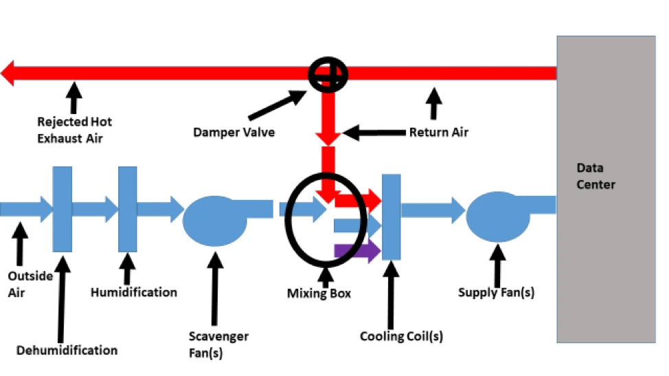
Figure 3: Simplified Air-Side Economizer
Other possible variations might be that the supply fans could all be integrated into precision CRAH units located inside the data center white space, along with the cooling coils; however, it is my recommendation that it is typically a superior design for the cooling coils and air movement mechanism to be integrated into the economizer. Besides typically superior efficiency of the larger fan systems, the integrated units are not adding fan energy heat load to the total data center cooling load. Missing from the illustration is the rest of the mechanical plant connected to the illustrated cooling coils. While this mechanical plant could be your typical chiller and tower set-up, it is often more practical to have integrated DX cooling with the economizer. After all, if the mechanical cooling is only required for 5-20% of the year, any DX inefficiency would be easily offset by the capital investment savings of DX cooling integrated into the economizer versus a separate chiller and heat rejection solution. Another variation might be the addition of a heater prior to the humidification and de-humidification stations. Such heaters historically functioned to help with de-humidification, though that practice is no longer recommended and is, in fact, illegal in some states. However, in extremely cold locations where re-cycling 100% of the data center return air into the mixing box might still be inadequate to get the supply temperature above the required minimum temperature, some heating of the ambient air is still more energy efficient than running the full mechanical plant.
There are just a couple more data points that need to be clarified prior to wrapping air-side economization into its own algorithm. First, the choice of humidification technology covers a wide variation in energy efficiency. Table 3 provides some general ballpark numbers for different types of humidification remediation, but your mileage may vary so it’s a good idea to get specifics from the equipment vendor.
Humidifier Energy Consumption | |
Type | kW/lbs/h |
Gas Fired | 0.390 |
Electrode | 0.333 |
Resistive | 0.333 |
Ultrasonic | 0.023 |
High Pressure Atomizing | 0.002 |
Table 3: Energy to Produce a Pound of Water Vapor per Hour3
Finally, we want to convert the dew point data we collected for the modification to the look-up table in Table 1 where we added columns for each possible dew point and were therefore able to derive annual hours for each dew point temperature. Then we want to convert those hours into pounds of water. There are several ways to get this done. I have just created a look-up table with the weight of moisture per cubic foot of air at sea level for every dew point from 32˚F to 120˚F (see Table 4 for a sample excerpted from that look up table) and then I merely have to write a simple modification to my sum equation at the bottom of each column from the modified Table 1:
=((SUM(AB10:AB8770)))*Water!B2*$A$1
Where:
AB10:AB8770 = Sum of “ones” in a particular dew point column
Water!B2 = Cell with pounds of water per ft3 air from Table 4 look up table (example is 32˚F, i.e., 0.00030 lbs)
$A$1 = Cell where CFM air delivered to the data center is plugged
Temperature (˚F) | Water (lb/ft3) |
32 | 0.00030 |
33 | 0.00031 |
34 | 0.00032 |
35 | 0.00034 |
36 | 0.00035 |
73 | 0.00127 |
74 | 0.00132 |
75 | 0.00136 |
76 | 0.00140 |
77 | 0.00145 |
78 | 0.00150 |
79 | 0.00154 |
Table 4: Moisture Content at Different Dew Points (Look-up Table Sample Excerpts)
The second step has two parts:
Sum the column totals for every column below the minimum allowable dew point. For our purposes we will use the ASHRAE recommendation of 42˚F.
Sum the column totals for every column above the maximum allowable dew point. For the purposes of this series of blogs, we will use the ASHRAE recommendation of 59˚F
The final data point required for the algorithm is an energy value for humidification. Since we know a total amount of water that needs to be removed, and a total amount of water that needs to be added, and wet and dry bulb conditions, this data could likely be provided by vendors. There are multitudinous ways to remove water from the data center, though Table 2 provided some indication, we will typically be more engaged in adding water than removing it. Nevertheless, for these example calculations, I will use either condensing dehumidification provided through dedicated cooling units or a rotary desiccant dehumidifier. For the former, I am going to assume 2.4kW for fan energy per 13.75 pounds of water; your mileage may vary, plus additional mechanical plant cooling energy. For the latter, I am going to assume 4kW of fan power per 250 pounds of water. These systems have a much higher energy usage for fans and heater to produce an air stream to remove the moisture captured in the desiccant wheel, but I am going to assume the wheel is plumbed into the data center return air path to basically deliver that function for free.
The hard work is done. We can begin assessing alternatives per the following:
(SAT-CA) > Look up table for calculation of H
Q1 = (H*FE)+HuL*E1)+(DHuL*E2)
Q2 = MC(8760-H)
Where:
SAT = Supply air temperature
CA = Cumulative approach temperature (could be 0; should be no more than 2˚F)
H = SAT-CA will establish DB column head in Table 1 and H=column∑
Q1 = Cooling energy in economizer mode
FE = Total fan energy (.76 times horsepower times number of fans. Be sure to cube the percent utilization to get affinity law economies)
HuL = Total humidification load. Pounds of water that must be added from Table 1 worksheet
DHuL = Total dehumidification load. Pounds of water that must be removed from Table 1 worksheet.
E1 = Humidification energy. Use values from Table 3 if vendor information has not been identified
E2 = Dehumidification energy. Use 2.4 kW per 13.75 pounds for condensing or 4kW per 250 pounds for desiccant wheel if vendor information has not been identified.
Q2 = Total cooling energy without economization
MC = Mechanical cooling – If provide by a traditional chiller mechanical plant, use:
CP = (1-(LWT-45).024) (BPxCT)
Where: CP = Chiller plant power
LWT= Chiller leaving water temperature ˚F
BP = Base power (kW per ton @ 45˚F LWT)
CT = Chiller tons
If provided by integrated DX system, use vendor data.
There is everything you need to assess the impact of airflow management on total data center cooling costs coupled with airside economization or for assessing relative merits of airside economization against series or parallel water-side economization in the context of different climate conditions. Remember, in this particular exercise I am driving toward making some apples-to-apples comparisons based on living inside the ASHRAE recommended environmental envelope. For those readers who would venture into the ASHRAE allowable environmental limits, the energy requirements for cooling any space would decrease dramatically from these calculations. Furthermore, if any readers are entertaining operating within the parameters published by most IT equipment OEMs, there is a very high likelihood you can forego completely both capital and operating expenses for any compressor/refrigerant cooling…period. That point has been made in numerous previous pieces. For now, my intent in forthcoming pieces is to use these algorithms to compare different types of economizers in different climate conditions and then to wrap up the series with a couple discussions on some of the less-discussed elements of the total cooling solution for data centers.
1 “Cooling Efficiency Algorithms: Economizers and Temperature Differentials (Water-side Economizers),” Upsite Blog, November 7, 2018
2 “Cooling Efficiency Algorithms: Economizers and Temperature Differentials Water Side Economizers (Parallel),” Upsite Blog, January 2, 2019
3 “Waterside and Airside Economizers: Design Considerations for Data Center Facilities,” Yuri Y. Lui, ASHRAE Transactions 2010, Volume 116, Part 1, page 106

Ian Seaton
Data Center Consultant
Let's keep in touch!
0 Comments
Trackbacks/Pingbacks