This article is the first of a 7-part series exploring the efficiency drivers of the different elements of a data center mechanical plant. Algorithms on how to calculate certain variables will be presented in each article, concluding with a final algorithm of how they all fit together in the last article.

In a previous piece, I covered how we used top of rack server inlet temperature as the control point for supply air temperature settings and how we used the ΔT between the bottom server inlet and top server inlet, in conjunction with various static pressure differentials to control supply air volume delivery. I demonstrated how critical effective airflow management is to allowing the highest possible temperature and lowest possible airflow. That discussion centered on controlling air temperature set points and CRAH fan speeds. However, the data center mechanical plant is a complex ecosystem with many inter-acting variables, often with competing design objectives. A good design and an effective control methodology take into consideration the trade-offs of these competing elements.

On the one hand, all this is done for us by our architectural engineering resource and then by whatever management tool we have in place to operate the data center, so what exactly do we need to know about how all these pieces work together? If continuous improvement is not an organizational mission, then we probably know everything we need to know. However, if we have objectives to squeeze more points off our data center PUE or re-direct budget dollars from mechanical overhead to productive ITE, then some understanding of how to measure the effects of our efforts is going to be worthwhile. To that end, I will explore the efficiency drivers of different elements of the mechanical plant in a series of pieces and finally wrap up with an algorithm for how they all fit together. Today, I begin with the temperature differential between cooling unit entering water and cooling unit exiting supply air.

Coil Performance

Air handler coil performance is one of those variables that we should never have to think about since the CRAH vendors have worked it all out for us, except when we do. One of these metrics will be approach temperature as a product of pressure drop in the air across the coils. The vendors have those curves as a function of entering and leaving temperatures of water and air, so why should we be concerned with how those numbers are derived? Two reasons immediately occur to me. First, if we are in the planning stage for a new data center or optimization upgrade project, we will want to understand how our decisions about CRAH coil size and associated pressure drops relate to decisions about optimum chiller set points at peak load and at part-load, for example. On the other hand, if we are trying to optimally manage an existing installation with mechanical plant components from different vendors, we may want to verify the management system is making wise decisions or we may even want to build our own.

The elements of this algorithm are illustrated in Figure 1, where:

EWT = Entering water temperature to the cooling coil

LWT = Leaving water temperature from the cooling coil

RAT = Return air temperature from the data center

SAT = Supply air temperature to the data center

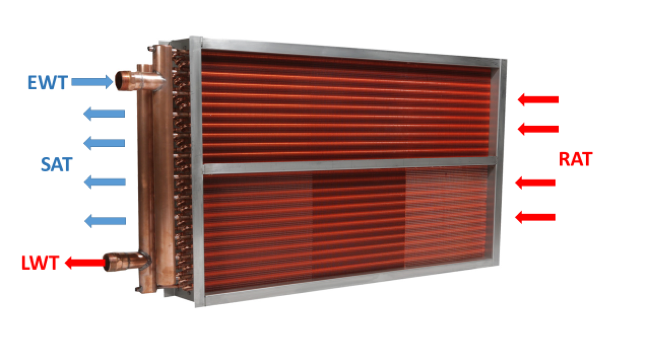
Figure 1: Variables Affecting Fan Pressure Drop Across Cooling Coils

The bigger the difference between EWT and SAT, the lower the pressure drop across the coils and we care because there is a nonlinear relationship between pressure drop and fan energy. As my regular faithful readers and any attendees of my data center efficiency classes know that fan motor energy is the cube of changes in fan speed, so also fan motor energy is the square of pressure drops, or conversely, pressure head increases result in a squared fan energy increase, assuming a fixed flow volume. For this variable, our algorithm would look something like:

A1=IF((SAT-EWT)≤4,0.5,IF((SAT-EWT)≤5,0.45,IF((SAT-EWT)≤6,0.4,IF((SAT-EWT)≤7,0.35,IF((SAT-EWT)≤8,0.3,IF((SAT-EWT)≤9,0.28,0.25))))))

Where:

A1   =   An Excel cell location for this answer. If this were a planning exercise, then we might have A1, A2, A3…A8760 and we might use historical hourly bin data to drive some of the other algorithms that produce SAT and EWT. If this were an operational control algorithm, then the level of granularity would be a management decision, with data collected by sensors.

4   = In the algorithm, these values could be 4-10 and these are ˚F. These values are hypothetical based on illustrative examples from the ASHRAE handbook, Best Practices for Datacom Facility Energy Efficiency. When possible, these values should be obtained from the cooling unit vendor.

A1   = The answer to this equation is going to be pressure in H₂O”.

Finding the Value

The second part of the economics of CRAH approach temperature and pressure drop is to find a value that can be dollarized and compared to the outputs of all other algorithms. In this example, I will solve for kW, which are easily dollarized.

POWER((A1/VR₁),2)*(.746*Hp₁)*AHUQ = kW

Where:

A1   =    The answer to the first half of the algorithm above (cells A1…A8760)

VR₁ =    Vendor pressure assumption for air handler fan performance (may be VR₂ etc.)

Hp₁ =    Total air handler fan motor horse power

AHUQ= Total quantity of air handlers on site

kW  =   Total kilowatts to operate CRAH fans at X approach (B1…B8760)

For future reference in a planning exercise, these kW answers would be recorded in cells B1…B8760. The sum of this column would be kW hours for a year. Different scenarios could be tested to determine most optimum design options. In an operational control exercise, each of these outputs would be evaluated in real time in relation to the outputs from other functions of the mechanical plant to dial in the most efficient combination of control settings.

Consider all Other Variables

When this particular algorithm is regarded in isolation, it is clear that the most efficient operation will occur with the highest approach temperature. When I was working in the data center lab at CPI, we typically operated with a 10˚F approach to our CRAHs and occasionally dropped that to 8˚F, raising our chiller LWT from 65˚F to 67˚F. Depending on where the supply air set point is, a lower approach temperature will reduce operating costs of the chiller and increase potential access to more free cooling hours. Therefore, the complete algorithm must take into account the economic impact of the competing variables to drive either the best design decisions or optimum operational settings. I will touch on other elements of the mechanical plant in subsequent pieces.