Cooling Efficiency Algorithms: Economizers and Temperature Differentials (Water-Side Economizers – Series)18 min read

In previous pieces I have discussed algorithms for accounting for the relationship between pressure drop and data center fan energy and the relationship between airflow management and chiller plant operating efficiency. Our conclusion so far has been that we looked at parameters with incompatible values – the approach temperature that benefits fan efficiency actually reduces chiller efficiency. With today’s blog I take up the first installment of a short sub-series looking at data center free cooling, after which we will roll these considerations up with chiller efficiency and fan efficiency. With the previous blogs, we saw that the algorithms for planning and operating had significant overlap and the tools could essentially be used for both purposes. With our look at free cooling, I will be focusing on planning, though the monitor and control implications will be apparent. I will address monitoring and control more directly after we have completed the planning piece, which is basically just a methodology for assessing the economic relative merits of different forms of free cooling.
While it may seem that the most economical form of free cooling is going to be to just open the window and let the hot air out, Figure 1 illustrates data for several U.S. sample cities that indicate at least availability is not quite so clear cut. The data represented in Figure 1 assumes excellent airflow management practices are in place and a 76˚F supply temperature is designed to maintain all server inlet temperatures within a 76-78˚F range, with some headroom to the ASHRAE recommended maximum threshold.
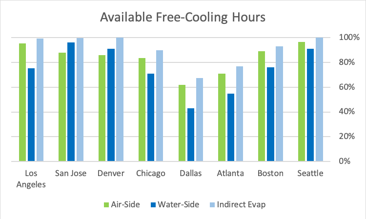
Figure 1: Free Cooling for Different Variations for Sample Cities, at 76˚F Supply Temperature
Figure 2 illustrates the importance of airflow management for any variation of economization in terms of maximizing the return on investment for free cooling as well as affecting the relative merits of different variations. With ineffective airflow management resulting in the requirement for a lower temperature set point, we can see a dramatic drop-off in available hours for free cooling.
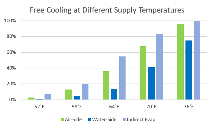
Figure 2: Free Cooling at Different Supply Air Temperatures, Los Angeles Example
As we can see in Figure 1, there are going to be variations in availability to different types of free cooling based on climate – no surprises there. In addition, as the Los Angeles example in Figure 2 illustrates, small changes in set points can make a big difference for some forms of free cooling and perhaps not so big differences for others. Therefore, a critical part of any planning exercise is to have access to reliable climate data. Hourly data is most relevant for a variety of reasons, such as the desirability of avoiding cycling a chiller on and off frequently. This data is available from various sources in various forms. Personally, I have organized data for several hundred NOAA stations in look-up tables that look like Table 1 below. Each cell in the Hours WB< and Hours DB< columns looks something like this: =IF(F724<$Q$9,1,0), so I can just reference the column header cells into any equation and it will calculate hours for any value I apply. Such tables will be integral to the algorithms I develop below and in upcoming pieces on the other variations of free cooling.
| Date | Time | Dry Bulb °F | Wet Bulb °F | Dew Point | Hours WB<37 | Hours DB<64 |
| 20070501 | 53 | 53 | 49 | 45 | 0 | 1 |
| 20070501 | 153 | 51 | 48 | 45 | 0 | 1 |
| 20070501 | 253 | 53 | 48 | 44 | 0 | 1 |
| 20070501 | 353 | 53 | 48 | 44 | 0 | 1 |
| 20070501 | 453 | 44 | 43 | 41 | 0 | 1 |
| 20070501 | 553 | 50 | 47 | 44 | 0 | 1 |
| 20070501 | 653 | 54 | 50 | 46 | 0 | 1 |
| 20070501 | 753 | 57 | 51 | 46 | 0 | 1 |
| 20070501 | 853 | 60 | 52 | 46 | 0 | 1 |
| 20070501 | 953 | 63 | 54 | 47 | 0 | 1 |
| 20070501 | 1053 | 65 | 54 | 46 | 0 | 0 |
| 20070501 | 1153 | 67 | 56 | 48 | 0 | 0 |
| 20070501 | 1253 | 67 | 57 | 50 | 0 | 0 |
| 20070501 | 1353 | 67 | 56 | 49 | 0 | 0 |
| 20070501 | 1453 | 66 | 56 | 48 | 0 | 0 |
| 20070501 | 1553 | 63 | 55 | 49 | 0 | 1 |
Table 1: Bin Data Look-Up Table, Sample Portion (Los Angeles)
Let us start with a water-side economizer, which can either have the economizer parallel to the chiller or in series with the chiller. In either case, we are exploiting cooler water tower temperatures to avoid running the chiller continuously. The series waterside economizer is illustrated in Figure 3 below. Please note this is not a complete engineering schematic as it is missing important valve and bypass elements; I am merely intending for this model to demonstrate location and functionality of energy cost-driving elements. The factors we will want to know, assume or verify include:
Sensible cooling load (basically UPS load + fan motors, etc.)
Supply air temperature
Ambient wet bulb temperatures (look-up table discussed above)
CRAH approach temperature (ΔT between supply air and coil entering water)
Heat exchanger approach temperature (condenser loop to data center loop)
CRAH fan energy
Pump energy
Chiller energy
Tower fan energy
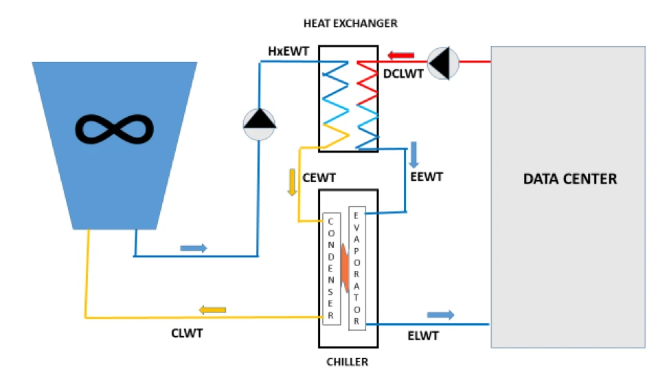
Figure 3: Series Water-Side Economizer
The elements of the series water-side economizer in Figure include the cooling tower and data center sandwiched around:
HxEWT Heat exchanger entering water temperature. This is the temperature of the water coming from the cooling tower. The tower approach temperature is the difference between this temperature and the ambient wet bulb temperature.
CEWT Condenser entering water temperature. This is the temperature of the cooling tower water after it has picked up the heat from the data center in the heat exchanger – typically plate and frame.
CLWT Condenser leaving water temperature. This is the temperature of the cooling tower loop/condenser loop after it has removed heat from either the heat exchanger or the chiller or both.
DCLWT Data center leaving water temperature. This is the data center chilled water loop after it has removed heat from all the CRAH unit coils.
EEWT Evaporator entering water temperature. If this temperature is lower than the maximum allowed supply temperature to the data center, then the chiller remains off. If this temperature is above the specified maximum data center supply (ELWT) but below the return (DCLWT), the chiller will operate at part load, delivering partial economization savings. If this temperature is at or above the expected DCLWT, then the chiller operates at capacity for full load.
ELWT Evaporator leaving water temperature. After the data center heat has been removed by either the heat exchanger or the chiller, this is the temperature that is being supplied to the data center CRAH coils.
Any algorithms for calculating economizer savings will need to take into account these elements. We presented a quick chiller energy calculation a couple weeks ago in, “Cooling Efficiency Algorithms: Chiller Performance and Temperature Differentials.” In that piece, I suggested:
CP = (1-(LWT-45).024) (BPxCT)
Where: CP = Chiller plant power
LWT= Chiller leaving water temperature ˚F
BP = Base power (kW per ton @ 45˚F LWT)
CT = Chiller tons
With this foundation, we can look at the actual economizer.
(SAT-CA) > Look up calculation for H
Q1 = H (CFP + PP + TFP)
Q2 = (8760 – H) (CP + PP + CFP + TFP)
Where:
SAT= Supply air temperature in the data center (See “The Shifting Conversation on Managing Airflow Management: A Mini Case Study,” Upsite blog)
CA= Cumulative approach temperatures (tower + heat exchanger or chiller + CRAH coils). SAT-CA will populate the cell at the head of the wet bulb column in the look up table.
H = Hours below the necessary wet bulb temperature to utilize free cooling. This number will be the sum (∑) of the hours under X˚F WB column in the look up table.
Q1 = Energy (kW Hours) annually to operate 100% free cooling
CFP = CRAH fan power, total in the data center
PP = Pump power, chilled water loop and condenser loop
TFP = Tower fan power
CP = Chiller power with no free cooling
Q2 = Energy (kW Hours) to operate mechanical plant with no free cooling
While that roll-up might look like we are done, we’re not. One of the real benefits of series water-side economization is that even when our hxEWT is too high to give us 100% free cooling, we can still get partial free cooling when the chiller entering water temperature (EEWT) is lower than the data center leaving water temperature (DCLWT), minus the cumulative CRAH coil and evaporator approach temperature, thereby reducing the load on the chiller. There are a variety of ways to sneak up on a partial free cooling estimate; one way would be to take advantage of the look-up table of bin data for the data center site.
IF DCLWT – (HxEWT + CA1) > 0˚F, then DCΔT- Value (=ΔT1)
PL1 = (DCCFM x ΔT1) ÷ 3140
PL2 = (DCCFM x ΔT2) ÷ 3140
PL3 = (DCCFM x ΔT3) ÷ 3140
PL4 = (DCCFM x ΔT4) ÷ 3140
Until every whole ˚F increment from 0 to Value has been accounted for
PLS1 = (PL1 ÷ Q) x CP
PLS2 = (PL2 ÷ Q) x CP
PLS3 = (PL3 ÷ Q) x CP
PLS4 = (PL4 ÷ Q) x CP
Then
Budget = Q1 + (Q2 – ((H1 x PLS1) + (H2 x PLS2) + (H3 PLS3) + (H4 x PLS4))
Where:
CA1 = Cumulative approach temperatures for heat exchanger and chiller
DCΔT = Difference between ELWT and DCLWT, i.e., the temperature rise of the data center (across CRAH coils)
Value = ˚F for calculating partial loads
ΔT1 = (i.e. VALUE) Difference between data center return water and condenser loop plus approach temperatures. Any value here represents opportunity for reducing chiller load and obtaining partial free cooling
PL1 = Partial load value #1in kW
DCCFM = Data center CFM (airflow demand)
PL2 = Partial load value #2 in kW (etc.)
ΔT2 = ΔT1 – 1˚F (and continue until 0)
PLS1 = Partial load savings for partial load value #1, etc.
Q = Data center total IT heat/power load
H1 = From the bin data look-up table: Total hours available for that one degree bucket, i.e. H+1
H2 = Total hours available from (H+1) to H+1+1, etc.
Budget = Total mechanical plant cooling energy budget with free cooling, partial free cooling and no free cooling with series water side economization at a particular load, particular supply air temperature, particular approach temperatures and particular IT load.
Next time I will look at parallel water-side economization, cover some basic differences between the parallel and series architectures and implementation implications, and explore some additional considerations with budgetary impacts, which are important though not necessarily directly in the operational expense realm. In addition, I will apply this little machine to the sample case study data center previously developed for the fan efficiency and chiller efficiency discussions. I suspect some of my readers may be surprised that such an exercise may not be quite as complicated as it may look on first blush here.

Ian Seaton
Data Center Consultant
Let's keep in touch!
0 Comments