Cooling Efficiency Algorithms: Economizers and Temperature Differentials (Water-Side Economizers – Parallel)22 min read

Next to powering all our IT equipment, powering the mechanical plant to cool all that IT equipment is the largest energy consumer in the data center and is frequently the main constraint to growth. Therefore, one might conclude that merely opening all the windows to let the hot air out and let cooler air in would provide the best path to energy savings and capacity optimization. One might be wrong. On the other hand, one might be right. My task in a series on cooling efficiency algorithms is to provide a roadmap for removing some of the guesswork in both design decisions and management practices. In September I covered cooling coil performance. In October I covered chiller efficiency. In November I began the conversation on free cooling, starting with water-side economization with economizer and chiller in series with each other, enabling periods of partial free cooling. In today’s piece, I will present algorithms for assessing the relative merits of water-side economization when the economizer (heat exchanger) and chiller are parallel, as illustrated in Figure 3. Upon completion of this series, we will apply these algorithms to a couple different scenarios to explore the variables which might make one model more attractive than another.
My rules of engagement will not change from the previous pieces in this series, so we can actually make some apples-to-apples comparisons when we get to the end. Therefore, we are assuming a data center with excellent airflow management practices in place that allow us to have a 76˚F supply air temperature capable of providing server inlet temperatures in a 76-78˚F range. With that 76˚F supply temperature, we can see in Figure 1 that in six cities we would have access to more free cooling hours with free air cooling than we would have with water-side economization. However, in Denver and San Jose we would have access to more free cooling hours with water-side economization. (Don’t worry: we will get around to indirect evaporative cooling before this series wraps up.) Nevertheless, access to hours does not necessarily directly correlate to energy use, hence the algorithm tools I am presenting.
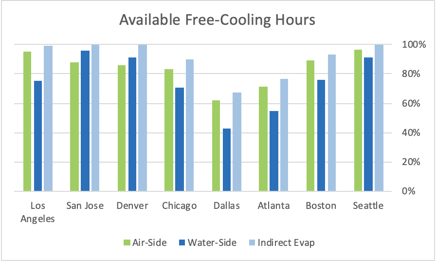
Figure 1: Free Cooling for Different Variations for Sample Cities, at 76˚F Supply Temperature
While my assumption about airflow management best practices and the resultant set point management flexibility may not change the relative merits of different variations of free cooling, it definitely moves the needle on whether or not free cooling should even be considered. Figure 2 illustrates access to free cooling hours at different levels of airflow management. Remember, before airflow management was everybody’s favorite topic at poker parties, BBQs, and happy hours, we saw return air set points around 68-70˚F, resulting in supply air temperatures in the 50-55˚F range. Therefore, the worst case number in Figure 2 (58˚F) still represents racks arranged in hot aisle – cold aisle and maybe some floor grommets and blanking panels deployed with random inconsistency, thereby allowing a 75˚F set-point resulting in 58˚F supply. Regardless, the free cooling hours data suggests pretty strongly that with less than optimum airflow management an investment in free cooling is going to be difficult to justify. With good airflow management, such investments are clearly in the no-brainer category.
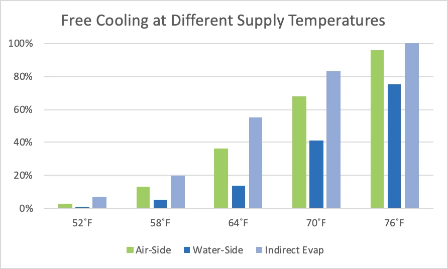
Figure 2: Free Cooling at Different Supply Air Temperatures, Los Angeles Example
A critical part of any planning exercise is to have access to reliable climate data. Hourly data is most relevant for a variety of reasons, such as the desirability of avoiding frequently cycling a chiller on and off . This data is available from various sources in various forms. Personally, I have organized data for several hundred NOAA stations in look-up tables that look like Table 1 below. Each cell in the Hours WB< and Hours DB< columns looks something like this: =IF(F724<$Q$9,1,0), so I can just reference the column header cells into any equation and it will calculate hours for any value I apply. There will be 8760 lines in each look up table. Be sure to closely scrutinize all the data you purchase. Not all weather stations are absolutely diligent in maintaining complete records. I guarantee you will find lines with no data recorded. My suggestion for you when you encounter these omissions is to enter values that fall halfway between the preceding data point and subsequent data point. While these estimates may cause you to miss some outliers, such as 1:53 am and 4:53 am in Table 1, the resultant exponential smoothing will still be more accurate than calculating all zeros for missing data points. Such tables were integral to the algorithms I developed for series water-side economization and will be for all subsequent discussions in this series.
| Date | Time | Dry Bulb °F | Wet Bulb °F | Dew Point | Hours WB<37 | Hours DB<64 |
| 20070501 | 53 | 53 | 49 | 45 | 0 | 1 |
| 20070501 | 153 | 51 | 48 | 45 | 0 | 1 |
| 20070501 | 253 | 53 | 48 | 44 | 0 | 1 |
| 20070501 | 353 | 53 | 48 | 44 | 0 | 1 |
| 20070501 | 453 | 44 | 43 | 41 | 0 | 1 |
| 20070501 | 553 | 50 | 47 | 44 | 0 | 1 |
| 20070501 | 653 | 54 | 50 | 46 | 0 | 1 |
| 20070501 | 753 | 57 | 51 | 46 | 0 | 1 |
| 20070501 | 853 | 60 | 52 | 46 | 0 | 1 |
| 20070501 | 953 | 63 | 54 | 47 | 0 | 1 |
| 20070501 | 1053 | 65 | 54 | 46 | 0 | 0 |
| 20070501 | 1153 | 67 | 56 | 48 | 0 | 0 |
| 20070501 | 1253 | 67 | 57 | 50 | 0 | 0 |
| 20070501 | 1353 | 67 | 56 | 49 | 0 | 0 |
| 20070501 | 1453 | 66 | 56 | 48 | 0 | 0 |
| 20070501 | 1553 | 63 | 55 | 49 | 0 | 1 |
Table 1: Bin Data Look-Up Table, Sample Portion (Los Angeles)
We will need the same data points for assessing a parallel water-side economizer as we used for building the algorithm for the series water-side economizer (“Cooling Efficiency Algorithms: Economizers and Temperature Differentials Water-side Economizers,” November 7, 2018). In both cases, we are exploiting cooler water tower temperatures to avoid running the chiller continuously. The parallel waterside economizer is illustrated in Figure 3 below. Please note this is not a complete engineering schematic as it is missing important valve and bypass elements; I am merely intending for this model to demonstrate location and functionality of energy cost-driving elements. The factors we will want to know, assume, or verify include:
Sensible cooling load (basically UPS load + fan motors, etc.)
Supply air temperature
Ambient wet bulb temperatures (look-up table discussed above)
CRAH approach temperature (ΔT between supply air and coil entering water)
Heat exchanger approach temperature (HxEWT to HxLWT in Figure 3)
CRAH fan energy
Pump energy
Chiller energy
Tower fan energy
Our methodology will be very similar, with two noteworthy differences. With series water-side economization, we get access to partial free cooling when our free cooling source water temperature is above the required supply temperature (minus associated approach temperatures) but below the return water temperature, which required our algorithm to monetize different degrees of partial free cooling in that range between supply and return temperatures. With the chiller and heat exchanger parallel to each other, there are two available conditions: chiller on and heat exchanger off or heat exchanger on and chiller off. Not having to account for the different degrees of partial free cooling would suggest that calculating parallel will be more simplified than calculating series, but we do have an added factor with parallel free cooling. We want to avoid the wear and tear on our chiller of hitting it with hard stops and starts, so our algorithm needs to take into consideration those climate conditions where the temperature hovers around our trigger temperature. In actual operation, this function is often manualized by an on-site engineer to monitor weather conditions on hourly forecasts to determine ambient conditions will stay below the trigger temperature long enough to justify shutting down the chiller and the eventual restart. For a planning decision algorithm, however, we need to be able to make reasonable estimates for when the trigger temperature really means it.
In addition, our assumption about excellent airflow management and resultant set points greatly simplifies both the modeling algorithm and the actual management of parallel water-side economization. Traditional standard practice dictated that tower water leaving temperature for the condenser (CEWT in Figure 3) could not be as cold as the water required for the economizer (HxEWT in Figure 3). In legacy data centers condenser minimum temperatures might be 55-65˚F whereas the economizer heat exchanger required water temperatures around 42-48˚F, thereby producing a chilled water loop (HxLWT) somewhere around 45-52˚F. There are three general design and management practices for accommodating these different tower temperature requirements. The simplest, though most expensive approach is to have a dedicated tower just for free cooling. This approach can be effective for upgrading a DX-cooled data center to free cooling with dual-coiled cooling units, but otherwise it is adding essentially a parallel infrastructure universe. Another approach is to add a bypass loop so the tower leaving water (CEWT) can be warmed by condenser return water (CLWT) or data center return water (DCLWT) to keep it at an optimum condenser temperature until it is cold enough to operate the free cooling heat exchanger and then switch over from the condenser to the heat exchanger. A third approach is to sacrifice free cooling hours by creating a deadband between the two systems. Fortunately, with excellent airflow management, the data center can operate with a chilled loop (ELWT or HxLWT) around 65˚F, allowing for a tower temperature of 62˚F (HxEWT), assuming a 3˚F approach temperature, which keeps us right in the middle of the condenser sweet spot and eliminates all the complicated work-arounds and extra expense for switching between the chiller and free cooling. In any case, when multiple chillers are in parallel with heat exchangers, the switch-over can be accomplished in stages to maximize access to free cooling and minimize hard stops and starts.
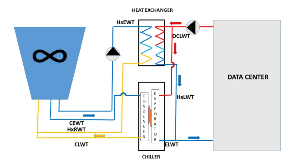
Figure 3: Parallel Water-Side Economizer
The elements of the parallel water-side economizer in Figure 3 include the cooling tower and data center sandwiched around:
HxEWT Heat exchanger entering water temperature. This is the temperature of the water coming from the cooling tower. The tower approach temperature is the difference between this temperature and the ambient wet bulb temperature.
CEWT Condenser entering water temperature. This is the temperature of the water coming from the cooling tower. The tower approach temperature is the difference between this temperature and the ambient wet bulb temperature. In legacy data centers CEWT must be 10-12˚F higher than HxEWT, but with excellent airflow management, that difference becomes minimal.
CLWT Condenser leaving water temperature. This is the temperature of the cooling tower loop/condenser loop after it has removed heat from the chiller.
HxRWT Heat exchanger return water temperature. This is the temperature of the cooling tower loop/heat exchanger loop after it has removed heat from the heat exchanger.
DCLWT Data center leaving water temperature. This is the data center chilled water loop after it has removed heat from all the CRAH unit coils. A valve will direct this water to either the economizer heat exchanger or the chiller evaporator, depending on which one is operating.
HxLWT Heat exchanger leaving water temperature. After the data center heat has been removed, this is the temperature that is being supplied to the data center CRAH coils.
ELWT Evaporator leaving water temperature. After the data center heat has been removed, this is the temperature that is being supplied to the data center CRAH coils.
Any algorithms for calculating economizer savings will need to take into account these elements. We presented a quick chiller energy calculation back in October: “Cooling Efficiency Algorithms: Chiller Performance and Temperature Differentials.” In that piece, I suggested:
CP = (1-(LWT-45).024) (BPxCT)
Where: CP = Chiller plant power
LWT= Chiller leaving water temperature ˚F
BP = Base power (kW per ton @ 45˚F LWT)
CT = Chiller tons
With this foundation, we can look at the actual economizer.
(SAT-CA) > Look up calculation for H
Q1 = H (CFP + PP + TFP)
Q2 = (8760 – H) (CP + PP + CFP + TFP)
Where:
SAT= Supply air temperature in the data center (See “The Shifting Conversation on Managing Airflow Management: A Mini Case Study,” Upsite blog)
CA= Cumulative approach temperatures (tower + heat exchanger or chiller + CRAH coils). SAT-CA will populate the cell at the head of the wet bulb column in the look up table.
H = Hours below the necessary wet bulb temperature to utilize free cooling. This number will be the sum (∑) of the hours under X˚F WB column in the look up table. The one complication for parallel versus series is that we may not want to count only one or two hours that dip below our trigger temperature if we don’t want to exercise our chiller with a lot of off/on cycling. If we say the wet bulb 1/0 column in Table 1 is column F and we want to have at least five hours of free cooling before we power down chillers, then we could add an additional column to our look-up table (H) and we could tabulate our free cooling hours with an equation like:
=+IF(OR(AND(H3=1,F4=1),AND(F4=1,F5=1,F6=1,F7=1,F8=1)),1,0), and copy that down the 8760 rows. The five elements in the second OR proposition could vary higher or lower depending how many hours of free cooling you prefer to get when you cycle chillers on and off.
Q1 = Energy (kW Hours) annually to operate 100% free cooling
CFP = CRAH fan power, total in the data center
PP = Pump power, chilled water loop and condenser loop
TFP = Tower fan power
CP = Chiller power with no free cooling
Q2 = Energy (kW Hours) to operate mechanical plant with no free cooling
The important differences between series and parallel water-side economization are:
Series provides access to additional partial free cooling hours
Parallel provides a more straightforward path to retrofitting an existing facility
Series energy estimates require weighing impact of partial free cooling
Parallel energy estimates require weighing allowable on/off cycle increments
Before developing some actual cooling cost estimates, next time we will review requirements for developing air-side economization algorithms for making energy use estimates, and then we can apply the various models to explore the relative operating cost benefits of different types of free cooling in different environmental conditions.

Ian Seaton
Data Center Consultant
Let's keep in touch!
Hello,
I am currently doing a masters degree in (M. Sc. A) related to cooling towers, in partnership with companies based in Quebec. We are working on highly anti-microbial and hydrophobic coatings and their potential application in Cooling Towers.
As a second task, I am building an Economic model that aims at predicting cooling tower costs based on parameters, such as usage&system design, weather, water quality. etc. All this to know whether a new technology is economically viable. What I need is Data. I am looking for companies who may posses large amounts of Data on Cooling towers : Location, hourly data: Temperatures, Water Flow (load) ,Conductivity, chemical feeds, costs. Anything that can help. I hope to do big data analytics using Python. In return, I’d gladly share my thesis hoping it can bring any important result relevant to the industry.
Hoping that you would have some data to help me produce some quality work,
Alexis Nossovitch