Specifying High ΔT Servers vs. Low ΔT Servers11 min read

Specifying computer equipment for a data center, might on the surface, appear to be one of the most basic of IT activities, however it can also have a profound impact on the data center mechanical plant and the overall cost of operations. There are many aspects to the decisions concerning the variety of computer servers and associated equipment that might be deployed in a data center, all of which have some degree of impact on the efficiency of the mechanical infrastructure. (For example, specifying traditional discrete servers versus blade servers is just one of those decisions). The IT decision process might typically focus on which type of server may best support virtualization or application segregation, or which may offer an easier path to technology refreshes for higher transaction speeds, or perhaps weigh the importance of I/O expansion scalability versus raw computing power. In addition, the effect on the total architecture of the data center should also be part of that decision process.
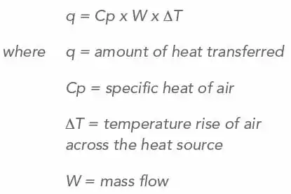
Historically, blade servers have produced higher ΔT’s than traditional rack-mount servers, popularly referred to as “pizza box” servers. That is to say, the cool supply air entering a blade chassis would exit as hotter air than would the supply air entering a pizza box server. This difference is described by the basic equation of heat transfer:
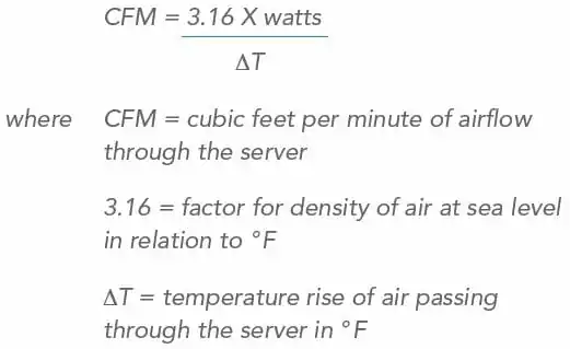
When we normalize the terms for our comfort zone of familiarity, this relationship is described as:
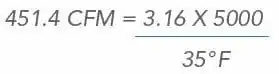
Based on this relationship, a 5kW blade server chassis with sixteen (16) servers and a 35° F ΔT would draw 451.4 CFM
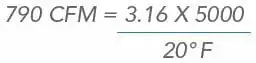
whereas ten (10) 500-watt pizza box servers with a 20° F ÄT would draw 790 CFM.
In a data center with 1600 blades (100 chassis), the servers would consume 45,140 CFM of chilled air (100 X 451.4) as opposed to a data center with 1000 pizza box servers, which would consume 79,000 CFM of chilled air. There are several ramifications to this airflow consumption difference. First, there would be a significant cooling unit fan energy savings in the data center with higher ÄT computer equipment. For example, if we specified 30-ton computer room air handlers (CRAH) with capacity to deliver 17,000 CFM each, we would need five CRAHs to meet the 79,000 CFM requirement. Naturally, those five CRAHs would be significantly over capacity for the lower airflow requirement of the higher ÄT data center, but fan affinity laws mean an even greater energy savings is achievable than might be expected in a straight linear relationship.
Those relationships are described by the equations:

Therefore, at 100% fan speed, 100% of the rated airflow volume is delivered, and at 50% fan speed, 50% of the rated airflow volume is delivered. Likewise, at 100% fan speed, 100% of the rated fan energy is consumed, but at 50% fan speed, only 12.5% of the rated fan energy is consumed, i.e., (1/2)3 = 1/8, or .125.
For the sake of discussion, then, let’s assume the 30-ton CRAHs in the example have approximately 12 horsepower motors rated at 9kW. The five CRAHs can produce 85,000 CFM (5 X 17,000), but only 79,000 CFM is actually required, so the variable air volume fans (either variable frequency drive [VFD] or electronically commutated [EC or “plug”] fans) could be turned down to 93%, or 15,800 CFM each, to meet the server requirements. At this flow or rpm level, each CRAH would be drawing 7.2kW:

With five CRAHs running 8760 hours a year, therefore, the blade data center would require 59,000 kW hours for cooling and the pizza box server data center would require 315,360 kW hours for cooling, or an 81% cooling energy savings for the data center with the servers with a higher ΔT.
While such an “apples-to-apples” comparison is useful for illustrating relative differences, such a comparison is more hypothetical than real. In reality, a more likely for the example scenarios would be that six 30-ton CRAH units might be deployed for the pizza box data center to provide a N+1 availability hedge and four of the same CRAHs would provide the same N+1 redundancy for the data center with the higher T equipment. In this case, a total cost of ownership calculation would include the difference of purchasing an additional two CRAHs and then the energy required to power those CRAHs in each scenario per year, per technology refresh cycle or per the estimated life of the data center, whichever metric is most relevant to the particular business model.
In addition to directly impacting the energy required to produce and move cooling air in the data center, the decision to specify blade servers or pizza box servers can also have an effect on the performance of an economizer or free cooling facility. Free cooling is discussed in more detail in our IT Decisions White Paper, but for the purposes of this discussion let’s consider an airside economizer and a set point for 68° F supply temperature delivered into the data center. Everybody understands that as long as the outside ambient temperature is below 68° F, we can use that air to cool our data center and save the energy required to remove the heat from the data center air and return the chilled air to the data center.
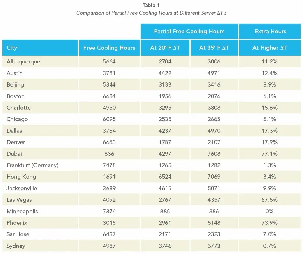
Next to the energy required to power the data center’s IT equipment, the single largest component of the data center operating budget is mechanical cooling, whether that is a centralized chiller plant or discrete DX CRAC units on the data center floor. Besides eliminating this mechanical plant expense when the ambient conditions are at or below the desired supply air temperature, there is a more or less linear partial reduction of those mechanical cooling costs whenever the ambient condition is lower than the data center return temperature. In the current example, therefore, there would be some partial free cooling benefit in the pizza box server data center as long as the external ambient conditions were below 88° F and in the blade server data center as long as the external ambient conditions were below 103° F (68+20 and 68+35, respectively).
Table 1 demonstrates that this value of additional partial free cooling hours will vary greatly based on the location of the data center and, by implication, also by the operational set point.
Just a few years ago, industry experts could confidently base analyses and energy use forecasts on 20° F as a standard ΔT for rack mount pizza box servers and 35° F as a standard ΔT for blade server systems. The playing field, however, has evolved over time. Server manufacturers continue to endeavor to produce more energy efficient servers. Much of this design energy is focused on microprocessor cores and software that slows down the computer when it is not working at high activity levels. Nevertheless, some of this work is also focused on the operating temperature specifications of internal components, resulting in reduced airflow requirements and higher allowable ΔT’s. Therefore, while the general distinction between pizza box servers and blade servers is still typically valid, it is not an absolute rule, so the specifying effort to exploit this element should require the server vendor to provide either ΔT information or CFM per kW ratios. Only by considering this element of a server specification can the server acquisition and deployment activity treat the data center as a totally integrated eco-system.

Ian Seaton
Data Center Consultant
Let’s keep in touch!
Airflow Management Awareness Month
Free Informative webinars every Tuesday in June.
0 Comments