Cooling Efficiency Algorithms: Encroaching into the Allowable Data Center Temperature Envelope23 min read

In this long series on cooling efficiency algorithms dating back to last September, I have presented tools for quantifying the energy use impact in the data center of:
Pressure and temperature differentials across cooling coils
Temperature differentials delivered to chillers
Temperature differentials and series water-side economizers
Temperature differentials and parallel water-side economizers
Temperature differentials and air-side economizers
Temperature and pressure differentials across condensers
Temperature and pressure differentials with heat exchangers
I developed these algorithms to answer two related questions:
- Should I design my data center with A or B?
- Should I manage some function to set point X or set point Y?
Some of these algorithms address both questions and some address one or the other. The list of algorithms is not necessarily intended to be all-inclusive, though for most of us this is really all we need to know. For some of us, I suspect we have already ventured into TMI territory. That being said, my base assumption through all of this was that we were going to operate our data center so our servers were living inside the ASHRAE TC 9.9 recommended environmental envelope (basically 64.4 – 80.6˚F). What happens if we choose to creep past that recommended barrier into the realm of allowable temperatures? The smart answer would be that if Professor Seaton built good algorithms, it should not make any difference. That would be the smart answer, but not necessarily the right answer.
The smart answer is that slipping past the recommended temperature boundary is already accounted for in the algorithms. For example, if we consider the pressure drop calculation in Equation 1, we merely allow SAT (supply air temperature) to creep up higher and we will still derive a pressure drop value that will drive our fan energy calculation.
If (SAT-EWT)<=4˚F, then A = 0.5” H2O, if not, then
If (SAT-EWT)<=5˚F, then A = 0.45” H2O, if not, then
If (SAT-EWT)<=6˚F, then A = 0.4” H2O, if not, then
If (SAT-EWT)<=7˚F, then A = 0.35” H2O, if not, then
If (SAT-EWT)<=8˚F, then A = 0.3” H2O, if not, then
If (SAT-EWT)<=9˚F, then A = 0.28” H2O, if not, then
Otherwise
A = 0.25” H2O
Where: SAT = Supply air temperature (from CRAH into the data center)
EWT = Entering water temperature (from chiller to CRAH coil)
X˚F = As noted from ASHRAE handbook, more precise values could come from equipment vendor
A = Pressure drop of air across CRAH coil
Equation 1: Pressure Drop at Different Approach Temperatures
Likewise, if we review the chiller energy algorithm from Cooling Efficiency Algorithms: Chiller Performance and Temperature Differentials, shown below in Equation 2, we see again that we merely need to plug in the higher LWT derived from a new maximum supply air set point. Simply, this LWT is the difference between an SAT minuend and approach subtrahend. That is to say, we calculate chiller energy use with leaving water temperature, which is the result of subtracting our cooling coil approach temperature from our data center supply air temperature. This equation works just fine with a 75˚F supply temperature, an 80˚F supply temperature or a 90˚F supply temperature.
CP = (1-(LWT-45).024) (BPxCT)
Where: CP = Chiller plant power
LWT = Chiller leaving water temperature ˚F
BP = Base power (kW per ton @ 45˚F LWT)
CT = Chiller tons
Equation 2: Chiller Plant Energy as a Result of Leaving Water Temperature
Similarly, the algorithm for calculating cooling energy use with water-side economization works just fine, regardless of how big a number is plugged in for the supply temperature. In Equation 3, we can see how the higher supply air temperature just provides access to a bigger number from the bin data look up table (see Cooling Efficiency Algorithms: Economizers and Temperature Differentials (Water-Side Economizers – Series) for an example of how to set up an easy-to-use look up table.). The bigger that number (wet bulb ambient temperature), the more free cooling hours, but the algorithm works as originally proposed, regardless of how high that temperature gets.
(SAT-CA) > Look up calculation for H
Q1 = H (CFP + PP + TFP)
Q2 = (8760 – H) (CP + PP + CFP + TFP)
Where:
SAT = Supply air temperature in the data center (see The Shifting Conversation on Managing Airflow Management: A Mini Case Study)
CA = Cumulative approach temperatures (tower + heat exchanger or chiller + CRAH coils). SAT-CA will populate the cell at the head of the wet bulb column in the look up table.
H = Hours below the necessary wet bulb temperature to utilize free cooling. This number will be the sum (∑) of the hours under X˚F WB column in the look up table.
Q1 = Energy (kW Hours) annually to operate 100% free cooling
CFP = CRAH fan power, total in the data center
PP = Pump power, chilled water loop and condenser loop
TFP = Tower fan power
CP = Chiller power with no free cooling
Q2 = Energy (kW Hours) to operate mechanical plant with no free cooling
Equation 3: Cooling Energy with Series Water-Side Economization
By now my observant reader may be wondering why we are having a special discussion about an algorithm for data center cooling for cases where we decide we are going to be OK slipping past the ASHRAE recommended temperature guidelines into the allowable range. After all, all our previously developed algorithms seem to function quite nicely, regardless of how we wander past that 80.6˚F threshold. It turns out, in reality, our cost saving trend line is going to look something like Figure 1, wherein we have a relatively linear descending cost line up to a point, and then our cost savings accrue a little less rapidly.
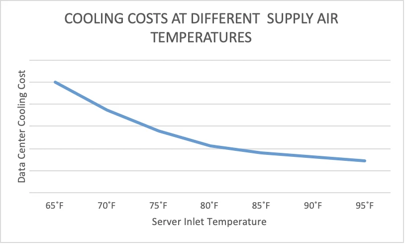
Figure 1: Relationship Between Cooling Cost and Supply Air Temperature
There are a variety of factors that reduce the trajectory of our cost savings trend line with increasing supply temperatures, but a key element is increased server fan energy at higher server inlet air temperatures. When this phenomena was first observed some ten years ago, happy hour conversations and even some experimental data suggested server fan energy actually reversed the total data center operating cost line somewhere between 77-80˚F. Unfortunately, the early experimental data came from tests that did not include economizers or chilled water plants and I corrected these misconceptions some four years ago in, Airflow Management Considerations for a New Data Center: Part 1 – Server Power vs Inlet Temperature.
SERVER ENERGY AT DIFFERENT TEMPERATURES | |||
Inlet Temperature | Server Energy Factor | Server Fan Flow Factor | CRAH Fan Power Factor |
68˚F | 100% | 100% | 1.00 |
72˚F | 100% | 100% | 1.00 |
77˚F | 101% | 103% | 1.09 |
81˚F | 102% | 106% | 1.19 |
86˚F | 103% | 109% | 1.41 |
90˚F | 105% | 114% | 1.48 |
95˚F | 107% | 119% | 1.56 |
99˚F | 110% | 126% | 2.00 |
104˚F | 113% | 132% | 2.30 |
Table 1: Effect of Increased Server Fan Energy at Different Inlet Temperatures on Server Total Energy
We will use the data from Table 1 to calculate server power at different inlet temperatures and CRAH fan power at different server inlet temperatures. Remember, if the server fans ramp up, we need to deliver a greater volume of air, even if it is warmer air, into the data center to meet the server air volume demand. The Server Energy Factor was derived from area plot graph Figure 2.7 in Thermal Guidelines for Data Processing Environments, p.27 and Table 2 from Airflow Management Considerations for a New Data Center: Part 1 – Server Power vs Inlet Temperature. This factor is a multiplier for total server fan energy at different server inlet temperatures and will be the factor used to calculate SP1, SP2, SP3, etc. in Equation 5 below. For example, based on Table 1 data, SP1 would be the total UPS server load with servers operating with 72˚F inlet air at typical work load times 1.01. (SP3, for example, = baseline server power times 1.03 for server inlet temperature at 86˚F) For design phase, the baseline number (at 72˚F) would come from the server manufacturer. The Server Fan Flow Factor is the increased airflow through the server at the higher power draw – this is the cube root of the portion of the Server Energy Factor committed exclusively to driving fans. Remember, our fan affinity law punishes us for flow increases just as non-linearly as it rewards us for flow decreases!
We will use the CRAH Fan Power Factor from Table 1 to calculate the impact on CRAH fan energy of meeting the increased demand from servers operating with higher inlet temperature air. First we need to know a baseline. If we are upgrading or fine-tuning an operating data center, then we just need to know the total CFM being produced and consumed. This total is not always that easy to come by, but can be calculated by the maximum CFM rating of your cooling equipment multiplied by the percent flow, which is going to be available somewhere on your CRAH control panels. For a new design, computational fluid dynamics will be our best bet. The model will tell us our total airflow demand and, using your airflow management assumptions, will tell us how much supply we will need to meet that demand, and keep all our servers operating at a happy temperature. Based on our server baseline data, we would want that CFD model to run with 72˚F server inlet air. Regardless how we obtain it, we start with a baseline total data center airflow, which will be some percentage of total capacity spread over all our cooling units. Remember, we like to stay under 80% capacity so we have some redundant capacity at hand for both emergencies and routine maintenance. Then Equation 4 provides us with our fan power kW for Equation 5.
FPB = Fan power baseline.
FP1 = FPB x 1.09
FP2 = FPB x 1.19
FP3 = FPB x 1.41
FP4 = FPB x 1.48
FP5 = FPB x 1.56
FP6 = FPB x 2.00
FP7 = FPB x 2.30
Where:
FPB = Fan power baseline, in kW. Total CRAH fan energy to supply 72˚F server inlet air and meet demand of all servers
FP1 = Total CRAH fan energy required to meet demand of servers with 77˚F inlet air
FP2 = Total CRAH fan energy required to meet demand of servers with 81˚F inlet air
And so forth from Table 1
Equation 4: CRAH Fan Power Correlations to Server Inlet Temperature
A side-benefit of calculating these CRAH fan power correlations derives from paying attention to the Fan Flow Factor column in Table 1. The airflow demand could surprise us with insights such as we could run out of redundant capacity at 85˚F or not have enough capacity period to meet demand at 104˚F. This is merely a cautionary tale – I have published earlier studies here that tell us we have very good pay-backs on adding cooling capacity to support higher temperatures. Remember – most of the year we are operating at much lower temperatures and banking all our fan affinity law savings.
With our server power figures and CRAH fan power figures, we can use Equation 5 to calculate our total energy adder for allowing our data center to occasionally creep into the allowable temperature area.
(FPB + SPB) (H ≤ Base)
Plus
(FP1 + SP1) (H1 – HB)
Plus
(FP2 + SP2) (H2 – H1+B)
Plus
(FP3 + SP3) (H3 – H2+1+B)
Plus
And so on until you hit the maximum server inlet temperature you will allow.
Where:
FPB = Base fan power. This is total data center CRAH fan energy to supply data center at baseline condition of 72˚F server inlet temperature.
SPB = Base server power. Total UPS server load when receiving 72˚F inlet air
H ≤ Base = These are hours of the year when server inlet temperatures will be equal to or less than the base condition, which in this case is 72˚F. In economizer mode, remember to count the hours when it is too hot for free cooling in either this bucket or whatever bucket includes your AC set point. See Table 2 for example of a look-up table copied from a NOAA data base.
FP1 = Fan power to support server demand at the first bin above base – in this case 77˚F
SP1 = Server power operating in the first inlet temperature bin above base (base server power X 1.01 per Table 1
H1 – HB = Hours of the year from the look-up table that that fall in the first bin above baseline – in this case 77-72
FP2 = Fan power to support server demand in temperature range of second bin above base (81˚F)
SP2 = Server power operating in the first inlet temperature bin above base (base server power X 1.02 per Table 1
(H2 – H1+B) = Hours of the year from the look-up table that that fall in the second bin above baseline – in this case 81-77
And so on until all the hours have been captured that fall under the maximum server inlet temperature that will be allowed.
Equation 5: Calculation for Total Fan Energy at Higher Inlet Temperatures
| Date | Time | Dry Bulb °F | Wet Bulb °F | Dew Point | Hours WB<37 | Hours DB<64 |
| 20070501 | 53 | 53 | 49 | 45 | 0 | 1 |
| 20070501 | 153 | 51 | 48 | 45 | 0 | 1 |
| 20070501 | 253 | 53 | 48 | 44 | 0 | 1 |
| 20070501 | 353 | 53 | 48 | 44 | 0 | 1 |
| 20070501 | 453 | 44 | 43 | 41 | 0 | 1 |
| 20070501 | 553 | 50 | 47 | 44 | 0 | 1 |
| 20070501 | 653 | 54 | 50 | 46 | 0 | 1 |
| 20070501 | 753 | 57 | 51 | 46 | 0 | 1 |
| 20070501 | 853 | 60 | 52 | 46 | 0 | 1 |
| 20070501 | 953 | 63 | 54 | 47 | 0 | 1 |
| 20070501 | 1053 | 65 | 54 | 46 | 0 | 0 |
| 20070501 | 1153 | 67 | 56 | 48 | 0 | 0 |
| 20070501 | 1253 | 67 | 57 | 50 | 0 | 0 |
| 20070501 | 1353 | 67 | 56 | 49 | 0 | 0 |
| 20070501 | 1453 | 66 | 56 | 48 | 0 | 0 |
| 20070501 | 1553 | 63 | 55 | 49 | 0 | 1 |
Table 2: Bin Data Look-Up Table, Sample Portion (Los Angeles)
While I burned quite a few words and lines of equations to get to this point, this is basically a pretty straightforward procedure, except for a couple complications. First, our table of NOAA temperature data does not directly correlate to server inlet air temperature. There are going to be some approach temperature subtrahends as well as airflow management inefficiencies to take into account. In addition, we could be looking at wet bulb ambient temperatures for water-side economizers and dry bulb ambient temperatures for air-side economizers. Therefore, when a calculation starts with server inlet temperature, we will want to hedge that by a few degrees to get to our required supply air temperature (SAT in the various equations). In a data center with excellent airflow management, that difference may only be 1-2˚F. In a data center with attention paid to airflow management but with some missing pieces or occasional lack of discipline, that difference may be 5-10˚F. In a data center with no regard for airflow management, that difference could easily exceed 20˚F, and this exercise would be basically pointless. Furthermore, not all servers are created equal. The factors used for these algorithms assume Class 3 servers with characteristics consistent with ASHRAE TC9.9 handbook examples, but your mileage could vary. Server fan energy was based on an assumption that server fans, operating at 50% as a default standard setting, consumed about 10% of the total server power draw. I have made all the calculations here as transparent as possible so if one of my readers has more accurate information on their own servers’ performance, then minor tweaks to the data in Table 1 would drive more accurate calculations.
We will give you a few weeks to digest this last installment, and then I will try to throw a rope around the whole series to summarize what should be the primary take-aways and then run a consolidated hypothetical case study. See you then.

Ian Seaton
Data Center Consultant
Let's keep in touch!
0 Comments