Heat exchangers refer to any kind of device used to transfer heat from one fluid to another fluid without direct contact between the fluids. Heated fluid flowing through one part of the heat exchanger transfers its heat to another cooler fluid or to the outside air. Heat exchangers are categorized by flow arrangement (parallel flow, counter flow or cross flow) and by the geometry of the core and fluid distribution elements. For us in the data center world, the most useful system of categorization is by the fluid heat transfer relationships, i.e., liquid-to-liquid, air-to-liquid, air-to-air, and air/liquid-to-evaporation. With this discussion of heat exchangers in the data center we are now just about six months into an extended series presenting various algorithms for either managing various elements of the mechanical plant or for planning capacity and operational budgets for the mechanical plant. I have previously hit the big ticket items of chillers, CRAHs/CRACs, air movement, and three different major approaches to free cooling, as well as some of the less discussed topics such as cooling towers, approach temperatures, coils and pressure drops, pumps, and dynamic redundancy. At this point, I would hope that some of my readers are muttering, “But Professor Seaton, heat exchangers typically don’t have any moving parts, so what would be in any algorithms and, more importantly, why should we care?” True enough, my friend, but as we discovered in our previous discussions of towers, condensers and coils, what goes on inside these mostly passive systems can have significant implications for both the effectiveness and efficiency of upstream and downstream systems.

There are certain key variables that will affect the performance of heat exchangers, regardless of the type of heat exchanger. The surface area of the core between the hot fluid and cold fluid and the flow rate of the fluids will establish the efficiency of the heat transfer and affect the operating costs of upstream and downstream systems. In addition, resistance to flow, the temperature difference between the two fluids, and approach temperature all factor into how the heat exchanger affects operating budgets for surrounding systems. Our algorithms will derive from these variables out to the moving parts for which they are key indicators.

Air-to-liquid heat exchangers are probably the most easily recognizable in the data center. These will include the coils in our CRAH (see Figure 1) and CRAC units as well as coils in rear door heat exchangers, top-of-rack heat exchangers and under-floor heat exchangers.

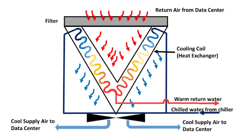
Figure 1: Air-to-Liquid Heat Exchanger Example (CRAH coil)

The bigger the difference between chilled water temperature entering the coils and the supply air temperature being returned to the data center, the lower the pressure drop across the coils. We care about this because there is a nonlinear relationship between pressure drop and fan energy. Just as fan motor energy is the cube of changes in fan speed, so also fan motor energy is the square of pressure drops, or conversely, pressure head increases result in a squared fan energy increase, assuming a fixed flow volume. For this variable, our algorithm would look something like:

A1=IF((SAT-EWT)≤4,0.5,IF((SAT-EWT)≤5,0.45,IF((SAT-EWT)≤6,0.4,IF((SAT-EWT)≤7,0.35,IF((SAT-EWT)≤8,0.3,IF((SAT-EWT)≤9,0.28,0.25))))))

Where:

The algorithm for dollarizing these pressure drop values is presented in Cooling Efficiency Algorithms: Coil Performance and Temperature Differentials.

Liquid-to-liquid heat exchangers include plate and frame water-side economizers (Figure 2) and condensers associated with chillers. Plate and frame heat exchangers utilize counter flow thereby allowing lower approach temperature differences, high temperature changes and increased efficiencies. The approach temperature in this case is the difference between the free cooling fluid temperature (aka the tower) and the chilled water temperature supplied to the data center. By optimizing all the elements of good airflow management in the data center we can operate with a much higher supply water temperature than we see in legacy data centers (65˚F is readily achievable) which, in conjunction with an approach temperature of only 1-2˚F, provides us access to significantly more hours of free cooling.

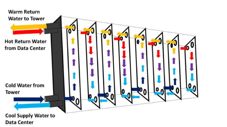
Figure 2: Liquid-to-Liquid Heat Exchanger Example (Plate and Frame Heat Exchanger, Exploded View)

The importance of a high supply air set point and minimal approach temperatures is clearly illustrated by the following excerpt from the economizer algorithms originally presented in Cooling Efficiency Algorithms: Economizers and Temperature Differentials (Waterside Economizers – Series).

(SAT-CA) > Look up calculation for H

                  Q₁ = H (CFP + PP + TFP)

            Q₂ =  (8760 – H) (CP + PP + CFP + TFP)

            Where:

SAT=     Supply air temperature in the data center (See The Shifting Conversation on Managing Airflow Management: A Mini Case Study)

CA=      Cumulative approach temperatures (tower + heat exchanger or chiller + CRAH coils). SAT-CA will populate the cell at the head of the wet bulb column in the look up table.

H =       Hours below the necessary wet bulb temperature to utilize free cooling. This number will be the sum (∑) of the hours under X˚F WB column in the look up table.

Q₁ =      Energy (kW Hours) annually to operate 100% free cooling

CFP =    CRAH fan power, total in the data center

PP =     Pump power, chilled water loop and condenser loop

TFP =    Tower fan power

CP =     Chiller power with no free cooling

Q₂ =      Energy (kW Hours) to operate mechanical plant with no free cooling

An air-to-air heat exchanger like the re-purposed energy recovery wheel, illustrated in Figure 3, is unique from the previously discussed heat exchangers because it actually has a moving part. This variation of heat exchanger includes a motor that rotates the wheel from the clean data center space to the more hostile ambient space allowing the data center heat captured in the wheel’s surface area (equivalent to the size of a soccer field) to be removed by the flow of cooler ambient temperature air. While this heat exchanger is therefore not a passive system, that motor is relatively small – a twenty foot diameter wheel is typically powered by a 1.5 horsepower motor and default maximum speeds are typically set at about 50%, resulting in about a 143 watt power load, similar to a couple old-style medium-brightness incandescent light bulbs. Other than that internal power use, efficiency algorithms for this heat exchanger will look at fan energy driven by the approach temperature through the wheel and the temperature difference between the ambient scavenger air and the data center supply air. This calculation is somewhat complicated by the internal controls that will rely as much as possible on the low energy consuming wheel motor before modulating fan speeds, but the vendors’ own calculators account for this as designed.

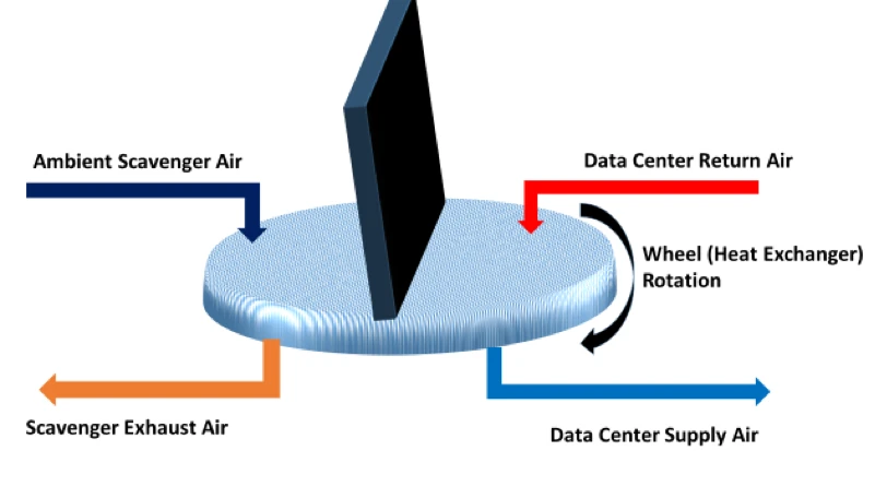
Figure 3: Air-to-Air Heat Exchanger Example (Re-Purposed Energy Recovery Wheel)

 Evaporative heat exchangers can be liquid-to-evaporation as in cooling towers as condensers or air-to-evaporation as in indirect evaporative coolers. An algorithm including tower approach and set point management was previously presented in Cooling Efficiency Algorithms: Economizers and Temperature Differentials (Waterside Economizers – Series). Operating conditions for evaporative heat exchangers tie to wet bulb ambient temperature rather than dry bulb conditions, but other than that we are still looking at approach temperatures, the data center ΔT, and the data center supply temperature, both of which are established by the quality of airflow management.

Other than the small motor for rotating air-to-air heat exchangers and pumps for scavenger spray on indirect evaporative cooling systems, heat exchangers are essentially passive elements of the total data center mechanical plant. Nevertheless, how they are sized and the temperature differentials supplied to them and that they supply to the data center all conspire to affect much bigger budgets with fan energy, chiller energy, economizer energy savings, and overall health of the data center. Where feasible, over-sizing is always a good idea to accentuate operational benefits of lower approach temperatures and fan and pump affinity law economies. Finally, none of these benefits can be fully realized without effective airflow management in the data center space.