Cooling Efficiency Algorithms: Condensers and Temperature Differentials22 min read

Over the past few months I have presented a series of algorithms for calculating the efficiency of different elements of the data center mechanical plant. These algorithms provided a framework for establishing trigger points for initiating different elements of the mechanical plant to optimize performance. For example, two sets of algorithms provided the basis for determining the relative merits of minimizing cooling coil approach temperature versus maximizing chiller leaving water temperature. I also provided examples of how to use these algorithms for evaluating the efficacy of competing design elements. At this point there is not much left to talk about. In fact, after the wrap-up on economizers three weeks ago, a very reasonable conclusion could easily be: Why all the bother about the mechanical plant? Who cares? We can operate within the ASHRAE recommended temperature ranges for such a large part of the year with free cooling, the refrigerant dinosaur is going to contribute such an insignificant portion of our total operating costs that it is hardly worth the effort to pay it any attention. In fact, if we stretch the boundaries of the ASHRAE guidelines in some cases to creep into what the ICT equipment manufacturers actually specify, less than 10% of the world’s data centers are built in locations that would necessitate any kind of air conditioning, for the equipment at least. Nevertheless, condensers are still an important (though less talked about) part of the cooling equation that should be discussed in some respects.
Out of sight, out of mind?
The condenser typically does not get a lot of air time in data center discussions for several reasons. It is typically the furthest removed from the white space, so there is always the “out of sight, out of mind” factor. Compared to the heavy hitters of ICT equipment, chiller and CRACs/CRAHs, the condenser doesn’t appear to mess with our bottom line that much. Besides being low on our radar, the condenser can also be extremely complicated, thereby making it easier for us to hand it off to the experts. In actuality, however, the condenser may have a larger impact on the data center’s total operating efficiency than we might at first think, but it is nevertheless a complicated system because of the multiple variables driving both correct sizing and efficient operation. For example, a ton of cooling is not a ton of cooling — we all know a ton equals 12,000 BTU hours; except a condenser ton equals 15,000 BTU hours because it is also absorbing the chiller heat load. Since I am not writing a condenser text book, I will be sinfully over-simplifying the subject in order to create a framework for relative scale in terms of the previous discussions on coils, chillers and economizers.
Types of Condensers and Their Impact on Efficiency
First, by “condenser” we mean the final heat rejection element of the mechanical plant. Heat sinks or cold plates absorb heat produced by ICT components. Air or water flows over those fins or plates to remove the heat from the ICT box. Heat will be removed from the data center air by cooling coils that transfer that heat to a liquid carrier that will go through another heat transfer at the chiller and will ultimately be rejected into the outside environment by the condenser. While there are a wide variety of condensers for different applications, in the data center world we typically use either a cooling tower (Figure 1) or a dry cooler (Figure 3).
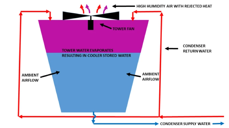
Figure 1: Simplified Schematic of a Data Center Cooling Tower
With a cooling tower, heated liquid is pumped from the chiller condenser element to the cooling tower where it is rejected via evaporation. The complete system is graphically illustrated in my previous articles on water-side economizers (Parallel and Series), which also explain one of the advantages of cooling tower heat rejection. When that condenser supply water temperature is at or below the temperature the chiller is supplying to the data center (minus a small heat exchange approach temperature), the chiller can be bypassed and shut down. In addition, cooling towers are more efficient than dry coolers in general, as indicated by heat rejection factors that add about 17% to a cooling tower load and 25% to a dry cooler load. Furthermore, I would always recommend over-sizing a cooling tower (minimal extra capital investment) to increase access to free cooling hours and also reduce tower fan and pump energy during normal condenser operation. A cooling tower efficiency number can be calculated by:
Q = (CR-CS)x100 / (CR-WB)
Where:
Q = Tower efficiency
CR = Hot condenser return water temperature
CS = Cold condenser supply water temperature
WB= Wet bulb ambient temperature
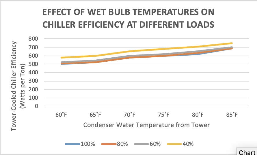
Figure 2: Chiller Efficiency as a Function of Ambient Wet Bulb Temperature
The cooling tower also affects chiller efficiency, as indicated in Figure 2, where we see operating energy levels for the chiller as a function of condenser supply water, resulting from ambient wet bulb conditions. Therefore, as with our water-side economizer calculations, we will want to have access to the same climate data for condenser calculations. Table 1 provides an example of an Excel worksheet format I use for compiling relevant NOAA hourly weather data to serve as look-up tables for efficiency calculations.
| Date | Time | Dry Bulb °F | Wet Bulb °F | Dew Point | Hours WB<37 | Hours DB<64 |
| 20070501 | 53 | 53 | 49 | 45 | 0 | 1 |
| 20070501 | 153 | 51 | 48 | 45 | 0 | 1 |
| 20070501 | 253 | 53 | 48 | 44 | 0 | 1 |
| 20070501 | 353 | 53 | 48 | 44 | 0 | 1 |
| 20070501 | 453 | 44 | 43 | 41 | 0 | 1 |
| 20070501 | 553 | 50 | 47 | 44 | 0 | 1 |
| 20070501 | 653 | 54 | 50 | 46 | 0 | 1 |
| 20070501 | 753 | 57 | 51 | 46 | 0 | 1 |
| 20070501 | 853 | 60 | 52 | 46 | 0 | 1 |
| 20070501 | 953 | 63 | 54 | 47 | 0 | 1 |
| 20070501 | 1053 | 65 | 54 | 46 | 0 | 0 |
| 20070501 | 1153 | 67 | 56 | 48 | 0 | 0 |
| 20070501 | 1253 | 67 | 57 | 50 | 0 | 0 |
| 20070501 | 1353 | 67 | 56 | 49 | 0 | 0 |
| 20070501 | 1453 | 66 | 56 | 48 | 0 | 0 |
| 20070501 | 1553 | 63 | 55 | 49 | 0 | 1 |
Table 1: Bin Data Look-Up Table, Sample Portion (Los Angeles)
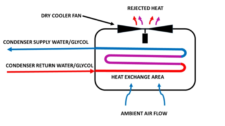
Figure 3: Simplified Schematic of a Data Center Air-Cooled Condenser
A dry cooler will typically set us back less than the initial capital investment for a cooling tower, though the efficiency differences typically give cooling towers a payback of less than one and a half years. Because of scale, however, dry coolers are often more suitable for smaller installations with lower IT loads and integrating with direct expansion cooling units. Dry coolers may also be attractive where the extra water use from tower evaporation plus blow-down and drift loss is either penalized or not allowed.
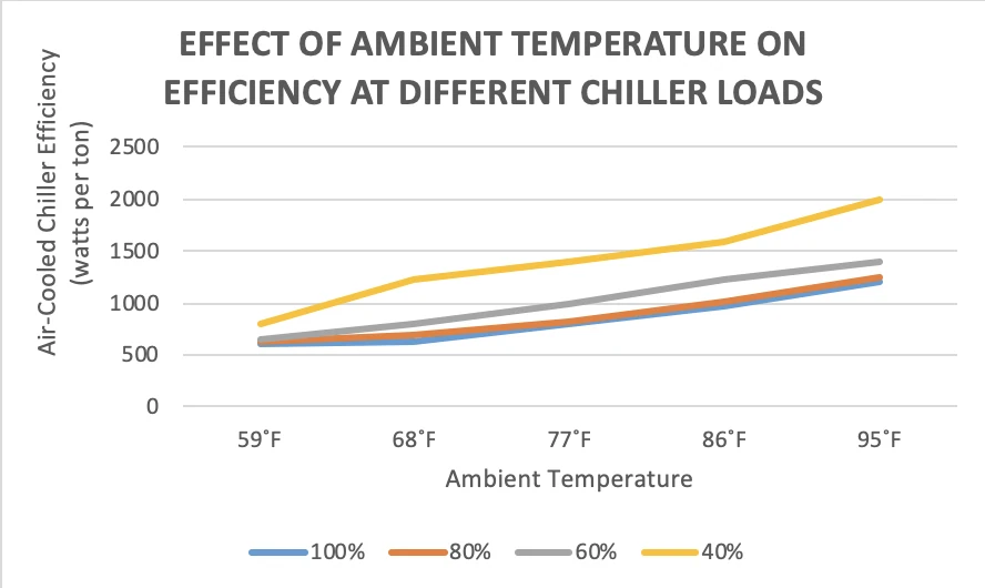
Figure 4: Chiller Efficiency as a Function of Ambient Temperature
In the same way wet bulb temperatures affect chiller efficiency with cooling towers, ambient dry bulb temperatures affect chiller efficiency in conjunction with dry coolers, as indicated by the data illustrated in Figure 4.
The energy consuming elements of the condenser are pumps and fans, regardless whether the condenser is a cooling tower or dry cooler. Energy variations, as implied by the above discussion, arise from having to increase fan speeds and pump throughput to compensate for higher ambient temperature conditions. Those potential efficiency losses can be mitigated by over-sizing the tower or oversizing the coils in a dry cooler. While the fan and pump energy savings may not offer a huge incentive for such investments, the effect of condenser operating points on overall chiller efficiency raises the importance of condenser efficiency.
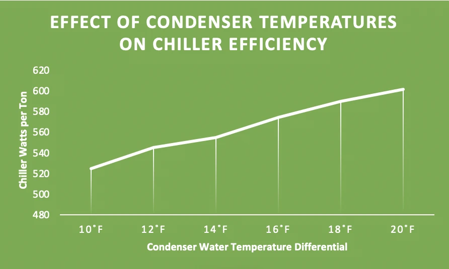
Figure 5: Chiller Efficiency as a Function of Condenser Water Temperature Differential
(Data from Best Practices for Datacom Facility Energy Efficiency, 2nd edition, ASHRAE, TC9.9, 2009, page 43)
The difference between the hot condenser return air and the cold condenser supply air, per the tower efficiency equation presented earlier also impacts chiller efficiency, as illustrated in Figure 5. In our one megawatt data center we have been using as a baseline through all these algorithm discussions, we would use over 240,000 kW hours more energy to operate our chiller with a 20˚F difference between tower entering and leaving water temperature than we would with a 10˚F difference. Such a reduction is a function of cooling tower size and fan and pump speeds.
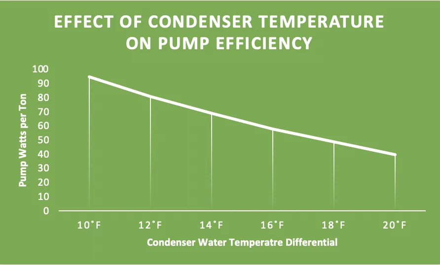
Figure 6: Pump Efficiency as a Function of Condenser Water Temperature Differential
We see in Figure 6 that pump efficiency is the inverse of chiller efficiency, as would be expected since increasing water flow and air flow will bring down the ΔT through the tower while obviously using more fan and pump energy. We would therefore expect the fan efficiency curve to resemble the pump curve. Our algorithm must take into account these competing functions. They do not just wash each other out as they are on different scales, which is clearly shown in Figure 7.
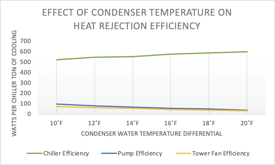
Figure 7: Mechanical Element Efficiency as a Function of Condenser Water Temperature Differential
Condenser Algorithm
While the condenser energy component is smaller than the other big hitters in the data center, it is particularly complex to accurately forecast because all the elements are variables. Granted, there is a nominal power rating for fans and pumps, but everything else is like nailing the proverbial jello to the wall. While we are outside of economization mode, the environment inside the data center should be relatively stable, i.e., X˚ supply air temperature and X+22˚ return air temperature and X-8˚ chiller leaving water temperature and (X-8˚)+12˚F chiller entering water temperature. However, on the condenser side we do not necessarily want to lock in our supply temperature because if we pick a number too low we will sacrifice pump and fan efficiency, but if we pick a number too high we will pass inefficiencies upstream to the chiller. By allowing that supply temperature from the condenser to follow Mother Nature, we can reap benefits of a low supply to the chiller without having to pay for maintaining a low ΔT through the condenser. Nevertheless, for a math model, we can’t have every element be a variable unless we want to do something like the Navier-Stokes equation approach for computational fluid dynamics where we keep recalculating all the variables until all the elements of the model harmonize. There are tools that will do that, but my goal here is to remain in the realm of Excel spreadsheets and bar napkins. Therefore, for the purposes of producing an output that will coordinate with the outputs of the previously developed algorithms for coils, chillers and economizers, we will approach this with the condenser cold supply being the variable, as a function of ambient temperature, and everything else remaining constant.
With that caveat, I propose:
Q = T (PN + FN)(HB)
+
Q1= T((PA1/PN)3 + (FA1/FN)3)(H1)
Where:
Q = Condenser energy at baseline (kW hours)
T = Tons cooling
PN = Nominal pump power (kW, speed = power at nominal)
FN = Nominal fan power (kW, speed = power at nominal)
HB = Hours at Condenser Return Temperature – 10˚ for baseline (look-up table)
WB for cooling tower and DB for dry cooler
Q1 = Condenser energy at second ambient condition
PA1 = Pump actual speed at second condition
FA1 = Fan actual speed at second condition
(Note: solve cube effect for fan and pump N(A/N)3
H1 = Hours at second condition (look-up table)
Notes:
- Continue solving for multiple Qs through range of ambient conditions.
- Use temperature look up table methodology described in previously cited economizer articles.
- Pick a temperature range for ambient conditions from baseline to lowest temperature, freezing or slightly above and divide your Q calculations into that many increments.
- We will revisit chiller efficiencies on final roll-up with effects of higher than baseline condenser supply temperatures.
- Determine fan and pump speed increments over range of ambient temperatures. For the data represented in Figure 6 and Figure 7, I used 5% per 2˚ Condenser manufacturer will have more precise ranges.
- For the baseline 1 MW data center I have been using as an example through this series, I used 95 watts per ton for a pump energy baseline and 75 watts per ton for a fan energy baseline. Dry cooler fan energy will generally be higher.
Cooling towers and dry coolers may not have all the appeal of virtualized servers, free cooling, liquid cooling or modular edge packages, but they play a critical role in the health of our data center eco-systems. Their impact on our operational bottom line extends beyond the limits of their immediate boundaries. We will explore that impact when we wrap this series up with some roll-ups of all the algorithms in a couple case studies. Meanwhile, coming up in the next few weeks I will touch on heat exchangers and extending the operating envelope, inter-mixed around a couple less intense topics.

Ian Seaton
Data Center Consultant
Let's keep in touch!
0 Comments